← All projectsAI · satellite + ocean data · iOS & Android
Shaka — a dive briefing for any point in the ocean.
Drop a pin on any patch of ocean — even a spot you keep secret — and Shaka reads that
exact point: satellite water clarity, swell bent around the real coastline, self-computed
tides, protected-area rules, AI-read fish intel. One 0–100 score. Nothing else scores an
arbitrary lat/long.
Product judgment under real constraints. The score is deliberately four factors — every factor that couldn't be measured honestly was cut, and when a data source dies the card says "Unavailable," never a plausible-looking default.
Full-stack range with AI-native tools. One person shipped the whole surface: Flutter apps on two platforms, a Kotlin/Ktor API fusing ~15 external sources, Python weather and tide pipelines, and a swell model calibrated against 4,700+ real spots.
An honest register. No uptime percentage ships without a defensible number; a weekly benchmark and a synthetic probe keep the forecasts honest, and the failures — like an eight-day silent stall — are told, not buried.
The live ocean map. Tap any point for an exact readout — "6.2 kts NNE", "2.7 ft" — pinch to zoom, switch layers.
The problem
Before a dive I'd open five tabs: swell, tides, water clarity, wind, and a fishing forum
for what's actually biting. None of them agree. None are pointed at the exact
patch of water I'm swimming into, and half are averaged across a whole region. Twenty
minutes of cross-checking later, I was still guessing.
The gap isn't a shortage of data — the ocean is heavily instrumented. The gap is that no
one fuses it down to a single point you choose. Swell forecasts ignore
the headland that shelters your cove. Tide tables snap to a gauge that might be forty
miles away. Fishing chatter buries one real catch under a week of noise. Shaka's job is
to collapse all of that into one honest read of one point.
Who it's for
Spearfishers, freedivers, surfers, boaters, shore anglers — anyone who cares about a
specific piece of ocean. The spot doesn't have to be a famous break in a public database.
Pin a reef you found yourself, save it as a private spot that's never shared with
anyone, and Shaka scores it like anywhere else. And that privacy is architecture,
not policy: no account, no email, no login anywhere in the product — spots sync against an
anonymous device ID, so your secret spot stays secret because there's no identity attached
to leak.
That's the hook. The places worth diving are the ones people don't post about.
Shaka is a phone-first field tool for that reality: power users pull up satellite clarity
layers and animated swell maps, casual users read the number and the color. Same engine
either way.
Product & journey
From an open map to a decision
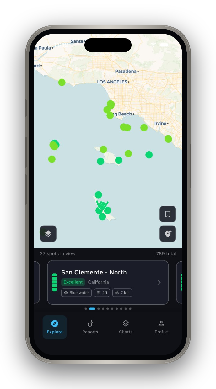
Everything starts on an open map. Browse a full screen of score-colored markers, or
long-press any patch of open water — a reef you found yourself, a ledge nobody posts
about — and Shaka scores a point that exists in no database. Save it as a
private spot: pinned and named to your profile, never surfaced to
other users.
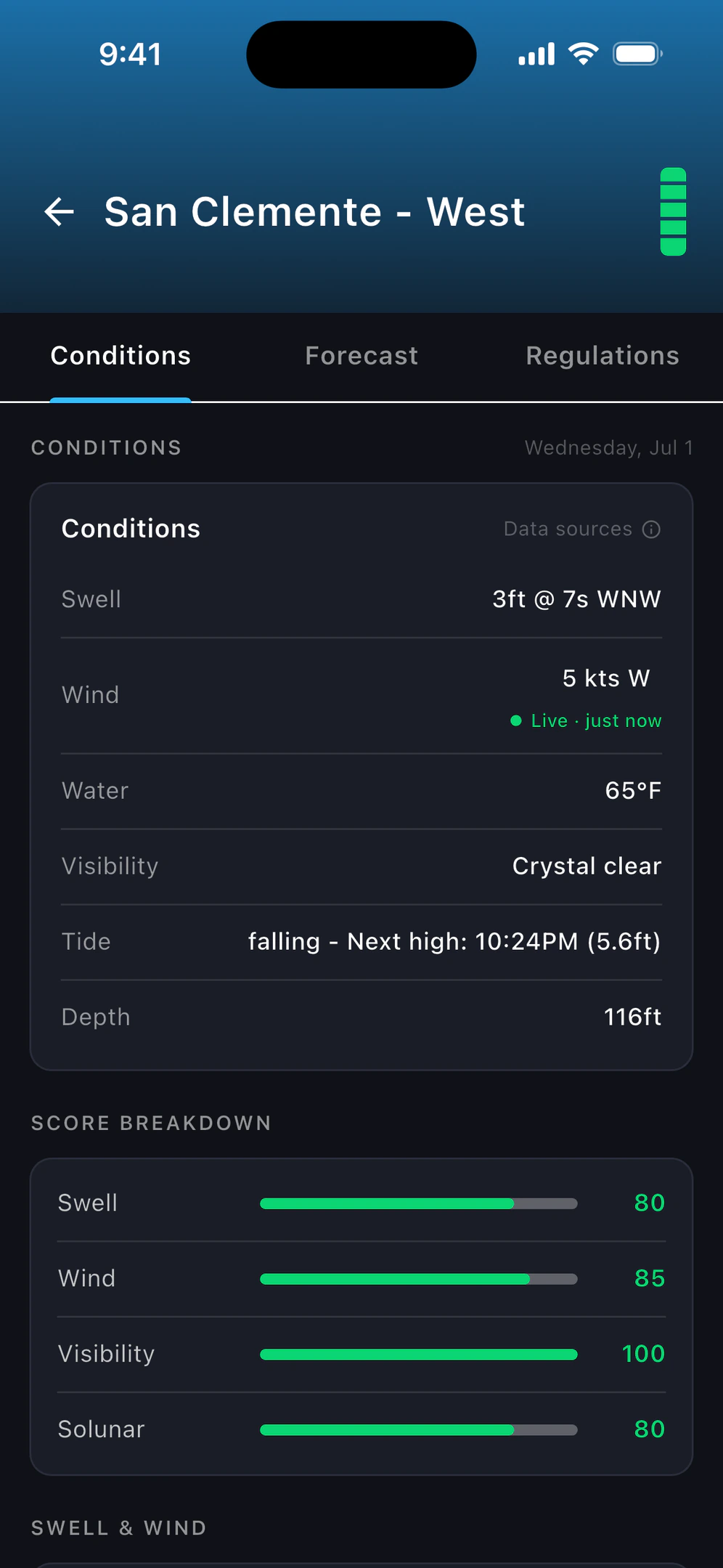
Tap a spot and the briefing opens: four tabs covering the score breakdown,
self-computed daily and weekly tides, the multi-day forecast, and the local rules.
From there you can pull up animated wind, swell, and current layers over satellite or
nautical basemaps, check NASA chlorophyll clarity from space to see the green plume
before you drive out, confirm whether spearfishing is even legal at the pin, and read
AI-summarized fishing reports that separate what was landed from what was merely
mentioned.
The hard part was making all of that feel like one calm surface instead of seven data
products stapled together — every layer has to work at any arbitrary point, not just
where someone installed a sensor. The payoff: twenty minutes of tab-hopping collapses
into one map, one tap, one number.
Explore — pan the scored map, tap a spot, get the briefing.
Design principles
Never fabricate data
Every other decision bends around this one. When a source goes dark, Shaka shows
"Unavailable" — never a plausible-looking default a user would mistake for
a measurement. Degradation is a contract: every upstream has a defined fallback, every request has
a per-source time budget, and a health endpoint gates features so a dead dependency
degrades one card instead of poisoning the whole score.
The rule is retroactive, too. Earlier versions had quietly filled gaps with climatology
defaults, so the cache now carries a hardcoded blocklist —
FAKE_CLIMATOLOGY_VALUES —
that recognizes those exact chlorophyll numbers and purges them on sight. I didn't just
stop fabricating data; I wrote code that hunts down what the system used to make up.
The score follows the same rule. It's a deliberately four-factor engine:
I cut every factor I couldn't measure honestly.
35%
Visibility — satellite chlorophyll-a
28%
Swell — coastline-aware wave height
22%
Wind — surface conditions
The remaining 15% is a solunar factor. Confidence decays in steps, not a
flat 10% a day: 95 for today, holding through the reliable near-term, down to 70 at a week
and 30 beyond three weeks, with an extra penalty for every missing core factor. If the
model doesn't know, the number says so.
Clean Ocean — the visual system
The interface runs on a system I call Clean Ocean: bright, confident data
on calm backgrounds. Scores pop; borders stay out of the way. Type is Inter. The palette
pairs an ocean-blue primary
(#1B6FA8) with a coral
secondary (#E8735A), on
warm off-whites and a warm near-black — easier on the eyes in bright coastal sun. The score
itself rides a five-tier, Apple-inspired palette from green
(#0BD674) to
red (#FF453A), so the
color tells you as much as the number.
Architecture & tech
The core is shaka-api, a Kotlin/Ktor + Exposed service on Railway. Its
clients fan out to a couple dozen sources, each behind its own rate limiter and circuit
breaker — one flaky upstream can't take the rest down. A DataPrefetch
jobs scheduler keeps two in-memory layers warm (SpotDataCache
and OceanDataCache),
backed by PostgreSQL/PostGIS. Two things run off the main service: a Python
weather pipeline that bakes Copernicus/ECMWF fields into RGB-encoded WebP
tiles on a Cloudflare R2 CDN, and a separate shaka-tide FastAPI service
that computes tides from the FES2022 model. The Flutter app reads all three directly.
Data sources
Satellite · weather
NASA GIBS · CMR Copernicus · ECMWF
Ocean · bathymetry
NOAA CO-OPS · ERDDAP NCEI · NDBC · GEBCO
Rules · fishing
ProtectedSeas · ArcGIS Global Fishing Watch
Reports · AI
SportFishingReport BD Outdoors · Groq
Utility APIs
Open-Meteo · Solunar · is-on-water
shaka-api · Kotlin/Ktor + Exposed
External source clients
Resilience layer
RateLimiter · CircuitBreaker per source · 3–30 s budgets
Ingest → cache/DB → API → app, with a cold-start loop that restores the full cache from Postgres on boot.
The load-bearing detail: the in-memory caches are the fast path, so a
cold start restores the full cache and hourly series from Postgres on boot —
a deploy no longer means a cold, source-hammering morning. How the rest of it stays fast
and stays up — the watchdog scheduler, the SLO engine, the per-source budgets — earned
its own section, next.
The quiet brief behind everything above: pull from roughly fifteen external sources —
NASA, NOAA, Copernicus, Open-Meteo, a self-hosted tide model, a fishing forum behind
Cloudflare — and deliver one number to a phone, fast, without ever falling over. Every
source is someone else's infrastructure having someone else's bad day, and a dive
briefing is only worth anything before the dive. So speed and reliability were
engineered as one system — and both were earned the slow way.
57 s → 3 s
One spot's ocean read — sequential, then parallel + cached
<100 ms
Cached spot detail — zero live API calls on the request path
99%
Per-job success SLO — below it, a run files its own breach report
Fast — stop asking the ocean at request time
The first version asked the ocean politely, one source at a time, and took
57 seconds to answer. Parallel fan-out and a TTL cache brought that to
2–5 s on a first call and under a second warm. The structural win came after:
background jobs pre-fetch every spot's conditions on staggered cadences, the whole cache
persists to Postgres and is restored on boot, and the request path stopped calling anyone
at all. Opening a cached spot today is a sub-100 ms read. Tides
take the idea to its logical end — the curves are deterministic, so each spot is
materialized a year deep exactly once and "now" is interpolated on read; collapsing the
old chart-plus-summary round trip alone bought back ~4.5 s. And the Groq-written
fishing insights left the request path the day one took fifteen seconds to generate and
the app timed out waiting. They're written after each scrape now; the request reads a row.
A brand-new pin is the one thing that can't be pre-fetched — the whole promise is scoring
a point that exists in no database. So creation fans out to every source at once, each on
its own clock: 3 s for SST, 15 s for the tide curve, a full 30 for NASA's
satellites. Each result writes to the cache the moment it lands, and the score
ships when the tide does — about two seconds in — while the stragglers back-fill.
Time-to-first-score fell from 15–45 s to 5–7 s.
Every source gets its own budget; the briefing ships the moment the tide lands, and the stragglers back-fill the cache.
The map got its own diet: weather layers render to lossless WebP (~30% smaller than PNG)
and ship from Cloudflare R2 behind an edge cache — tiles for six hours, the catalog for
five minutes — and the land mask that keeps wind particles off the beach went from a
3.7 MB GeoJSON on every load to 10–50 KB of PMTiles range requests per view.
None of this was designed up front; the git log reads like paid tuition. A 30-second
outer timeout raced the 30-second HTTP timeout inside it and lost by
84 ms, silently discarding good data. A five-connection DB pool let batch
jobs starve user saves. The tile endpoint advertised byte ranges while serving whole
files, which iOS does not forgive. Deploy warmup once ran every prefetch job
synchronously and took twenty minutes — deleted. Even the wind particles were tuned
twice: speed factor 8 read like a storm warning, so it ships at 3. Each fix is small.
The speed is their sum.
Reliable — alert on silence, not just failure
The failure that teaches you reliability is never a crash. Mine was a silent stall: a
hung dependency froze every background job mid-iteration, nothing crashed, so nothing
alerted — and for eight days the app served politely aging data. The scheduler that came
out of it treats a hang as the first-class failure. All twelve background loops run under
one supervisor (SupervisorJob),
every iteration inside its own
withTimeout, so a
stuck job forfeits one turn instead of its life. Starts are staggered across the first
fifteen minutes after a deploy, so a restart doesn't stampede fifteen upstreams at once.
Detection is its own machinery. Every job reports per-item results against a
99% success SLO; a run below it files a breach that names its own
dominant error — "Pattern: 7/9 failures are timeout" — instead of leaving me to diff
stack traces at breakfast. Failures fingerprint to stable Sentry issues, so one bad night
is one issue, not three hundred. Every run ships structured JSON to BetterStack, and each
job pings a heartbeat on success, so silence itself pages. On boot, an env audit
names which feature each missing variable would quietly degrade — half of all "outages"
are a renamed env var.
The perimeter is per-source, because the sources are nothing alike: token-bucket rate
limiters tuned to each provider (Copernicus gets 1 request/s and no benefit of the doubt;
Open-Meteo tolerates 5), circuit breakers that open after five straight failures and
probe again a minute later, and fetch budgets from 3 to 30 s depending on how slow
each source has earned the right to be. When something dies anyway, the degradation
contract holds: the card says Unavailable. What I won't print is an uptime percentage —
this monitoring is younger than the app, and I don't have a defensible number yet. Which
is also why a synthetic probe now walks the real user journey every 30 minutes: I stopped
trusting dashboards that don't open the app.
Challenging features
Scoring an arbitrary point means every layer has to work anywhere, not just where
someone installed a sensor. Six problems ate most of the engineering time. For each: what
I tried first, why it broke, where it landed.
1 · Mapping — scientific overlays, anywhere
Shaka lives on a map that carries things a normal map app never shows: animated wind
particles, swell-height rasters, current fields, satellite clarity plumes.
I started on Google Maps (google_maps_flutter)
and ripped it out entirely — a scientific overlay stack doesn't fit a locked-down,
per-load-priced tiling model. I moved to flutter_map over
OpenStreetMap for custom raster overlays and offline downloads, then consolidated the
interactive and animated maps on MapLibre GL. Not a from-scratch map
engine; custom overlays that grew into a MapLibre pipeline.
Basemaps are user-selectable and persisted via SharedPreferences:
a default Carto Voyager, a Satellite style (Voyager + ArcGIS World Imagery),
and a Nautical style (Carto Positron + ArcGIS Ocean + OpenSeaMap) for charts
and depth.
Map providers over time — a pivot, not a rewrite.
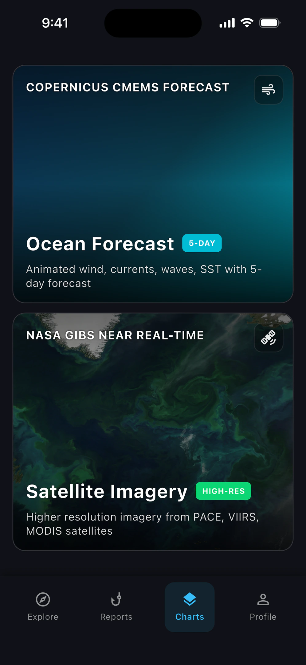
Animated weather maps bring the ocean to life — wind, currents, swell, and more as
vivid, interactive forecasts. I pull the model fields and render them into RGB-encoded
WebP "data textures" (a catalog.json
plus tiles) served from R2.
The hard part was making raw model output feel alive without melting a phone. Behind
the scenes the client stacks MapLibre GL + deck.gl + luma.gl +
weatherlayers-gl: wind and currents render as particle layers
(~10k particles, imageUnscale [-500, 500]),
while scalar fields like SST, wave height, chlorophyll, and salinity render as rasters
with per-layer palettes. Land masking draws PMTiles vector tiles back
over the particles so wind doesn't blow across the beach, and frames interpolate
between model timesteps for smooth motion.
The result: zoom into the smallest bay and watch the conditions you'd actually
navigate.
~10k wind particles, live — then the swell layer.
Ocean fields become RGB pixels, then particles and rasters — with land painted back over the top.
2 · Satellite rendering & water clarity
Visibility is the heaviest factor in the score, and it comes from chlorophyll-a: greener
water, shorter sightlines. Two independent paths feed it, and they stay distinct on purpose.
The first is NASA GIBS pixel-sampling — the same imagery you can scrub
through by date on the map, watching clouds move while the green plume stays put. Five
chlorophyll instruments feed it: PACE OCI, VIIRS on NOAA-20 and NOAA-21, and
Sentinel-3A and 3B OLCI.
The hard part is that GIBS serves pictures, not numbers. For each layer I hit
the WMS GetMap for a
tiny ~10×10 px box around the point, today and yesterday, and hand-decode
the PNG — parse IHDR/IDAT, inflate, honor each row's filter byte — to find the
first non-transparent pixel as a
#RRGGBB. An embedded
255-entry NASA VIIRS chlorophyll colormap turns that color back into a
concentration by nearest-RGB match (Euclidean distance, rejected past a threshold of 30).
The five satellites then fuse as a geometric mean of log-space
estimates, preferring a cloud-free reading from yesterday over a clouded one
today — so the map shows you the plume, and the score already knows it's there.
Scrubbing GIBS imagery by date — clouds move, the plume stays.
The second path is the trustworthy one. Copernicus Marine L3 NRT returns ZSD
(Secchi-disk visibility, in meters) and CHL as actual measurements, and returns
null under cloud rather than faking a value. An opt-in real-time path runs a Sentinel-3 OLCI
evalscript through the Sentinel Hub Process API. Priority: Copernicus CHL, then cached
ERDDAP CHL, then the GIBS estimate. GIBS colors are display-grade and prone to coastal
contamination — a last resort, never the headline number.
Two lanes into one honest number: measurements win, the pixel estimate is the fallback.
3 · Swell — bending the forecast around the coastline
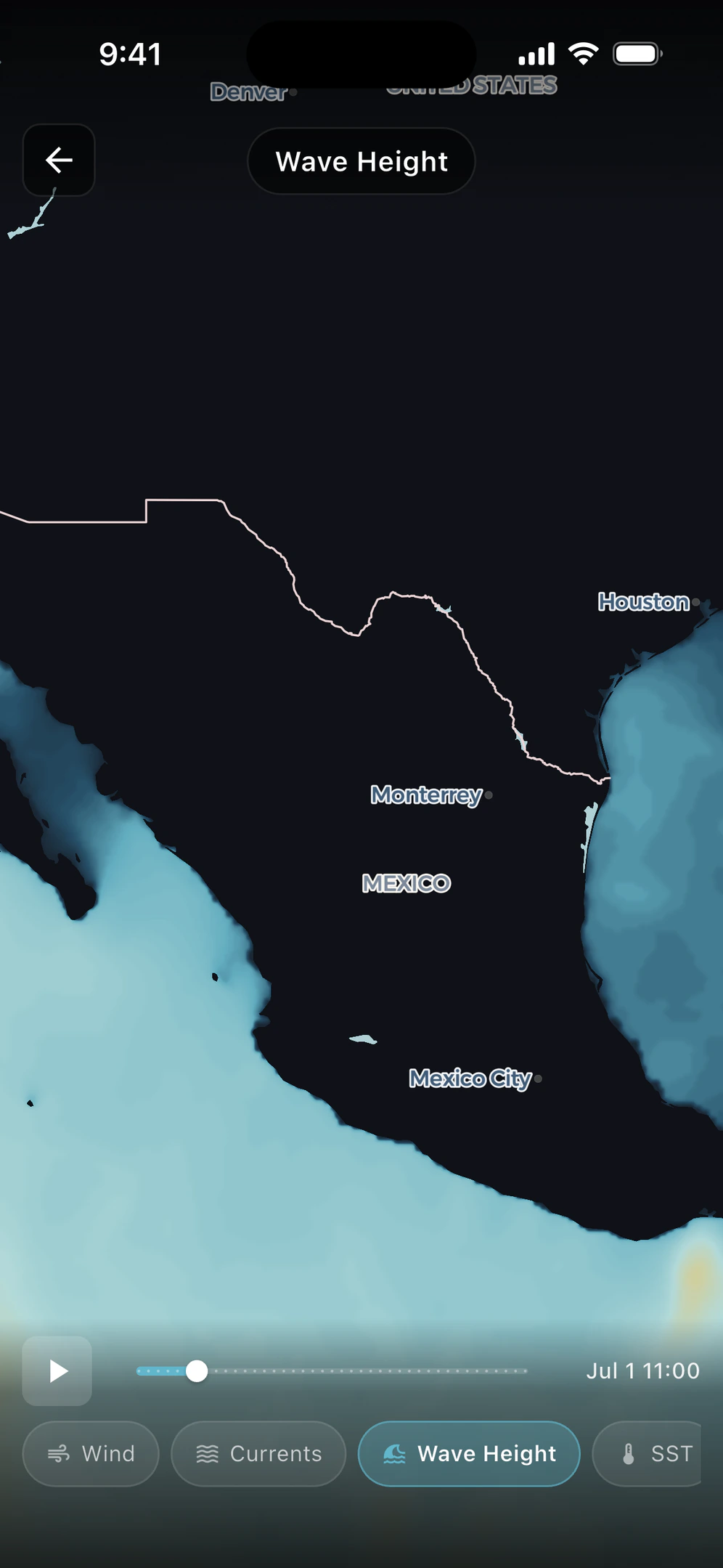
This is the feature the whole app is about, and the hardest. The wave-height layer
shows what the open ocean is sending — swell rasters you can scrub forward through the
forecast, straight from the model fields the weather pipeline bakes onto the map.
The hard part is that a global forecast only knows open water. It says nothing about
whether a headland shelters your cove, and the same offshore swell can be head-high at
one point and flat 300 m away. For a score pinned to an exact spot, the forecast
has to be bent around the real coastline.
So the raster is the honest starting point, and Shaka's own physics — exposure
ray-casting plus a calibrated attenuation model, below — decides how much of it
actually reaches your pin. The number the score uses is the sheltered one, not the
open-ocean headline.
The wave-height layer — open-ocean swell, before the coastline bends it.
The primary source is Open-Meteo Marine. A NOAA NDBC buoy
overrides it within 1.5 nm — that close, the buoy already reflects local conditions,
so no attenuation is layered on top. Everywhere else I compute the shelter myself.
Exposure profiling ray-casts 16 compass directions (22.5° steps) at 1, 2,
and 5 km rings — great-circle destination points — and asks a land/water API for the
nearest-land distance in each direction, or marks it OPEN. That profile feeds
Attenuation Model V2 at the swell's interpolated arrival bearing.
Exposure profiling: 16 rays × three rings decide how much open-ocean swell actually reaches the pin.
The model runs four stages on the arrival bearing: a land-distance factor
(0.492 at ≤1 km up to 0.954 in the open); a period modifier, because
long-period groundswell wraps around land better than short wind chop; an onshore
wind-sea term (windSea = √(total² − swell²),
added only when wind and swell align); and an offshore-to-surf scale of 0.690.
Secondary swell trains get the same treatment.
None of it counts without calibration. The constants were tuned with scipy's
differential evolution against 4,700+ Surfline spots and validated
on a held-out set: MAE 0.243 ft, 84% of predictions within half a
foot. A weekly GitHub Actions job re-benchmarks against Surfline (a Playwright scraper) and
streams the results to a BetterStack dashboard, so drift shows up as a chart, not a surprise.
MAE 0.243 ft · 84% within 0.5 ft — and a weekly benchmark that keeps it honest.
4 · Tides — any point, not the nearest gauge
NOAA CO-OPS was the obvious start, and the obvious dead end. It only knows tides at physical
gauge stations — inaccurate the moment you move away from one, useless
outside the US. So Shaka computes the tide itself. shaka-tide,
a Python FastAPI service, runs real harmonic synthesis on the FES2022
model (fes2022b ocean_tide_extrapolated)
via pyTMD, predicting the major constituents and inferring the minor ones, in the spot's
own timezone.
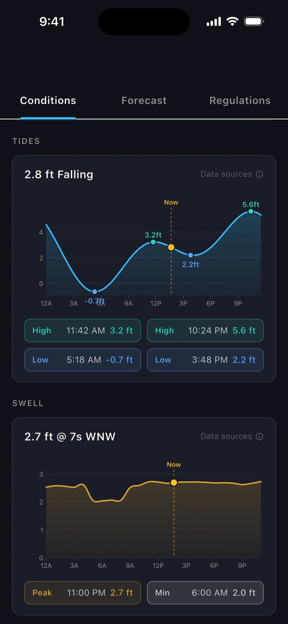
The tide tab gives you the curve for your exact pin — the current height, whether it's
rising or falling, and the day's highs and lows marked on the chart — not a reading
borrowed from a gauge forty miles away.
The hard part is honesty in the details. The raw model gives heights above mean sea
level; every chart a diver reads uses MLLW. I convert with a
precomputed global 0.5° MLLW offset grid, built from a full year of
hourly heights per cell. Highs and lows come out of a small extremes pipeline: find
local min/max, merge clusters within three hours, reclassify so highs and lows strictly
alternate, then filter by relative prominence adapted to the local tidal range.
Each spot is materialized a full year into Postgres rather than
recomputed per request; "now" is interpolated on read, and a monthly job tops up the
horizon. The payoff: the chart is instant every time you open it, anywhere on Earth.
The tide curve for the exact pin — highs and lows out of the extremes pipeline.
Per-point tide prediction — normally a paid capability — computed and cached for free.
The war stories are real. FES2022 holds a ~5 GB working set, which meant repeated OOM
crashes on Railway until I capped the service to a single warm instance
(concurrency=1) and pinned
pyTMD to 3.0.3. AVISO's FTP is flaky enough that I wrote a streaming, resumable downloader;
one model file took roughly 20 attempts over five hours to pull down cleanly.
5 · Rules & regulations — is spearfishing even legal here?
A dive score is incomplete if it can't tell you whether fishing is legal there. Rules come
from ProtectedSeas Navigator, a free Esri/ArcGIS Feature Service covering
70+ countries. One detail corrects my own README: the point-in-polygon containment runs
server-side in ArcGIS. I POST the point as an Esri geometry with
esriSpatialRelIntersects —
not local PostGIS, which handles spot search and fishing-report proximity
but not MPAs. Two calls go out: a 1,500 m buffer to catch nearby protected areas, and
an exact call to decide inside-vs-nearby.
The hard part: any ocean point sits under a stack of overlapping zones — EEZ, state waters,
sanctuaries, reserves. Relevance ranking cuts through it. Marine life conservation districts
rank first, then sanctuaries and reserves that prohibit spearfishing; purely jurisdictional
layers (EEZ, territorial, thrill-craft zones) get filtered out. What survives is sorted
prohibited-first, then by Level of Fishing Protection (LFP 1–5). The app surfaces the site
name, designation, spearfishing status, LFP, and species of concern, refreshed weekly.
Containment runs server-side in ArcGIS; relevance ranking turns a pile of zones into one clear answer.
6 · Fishing reports — real catches out of noisy chatter
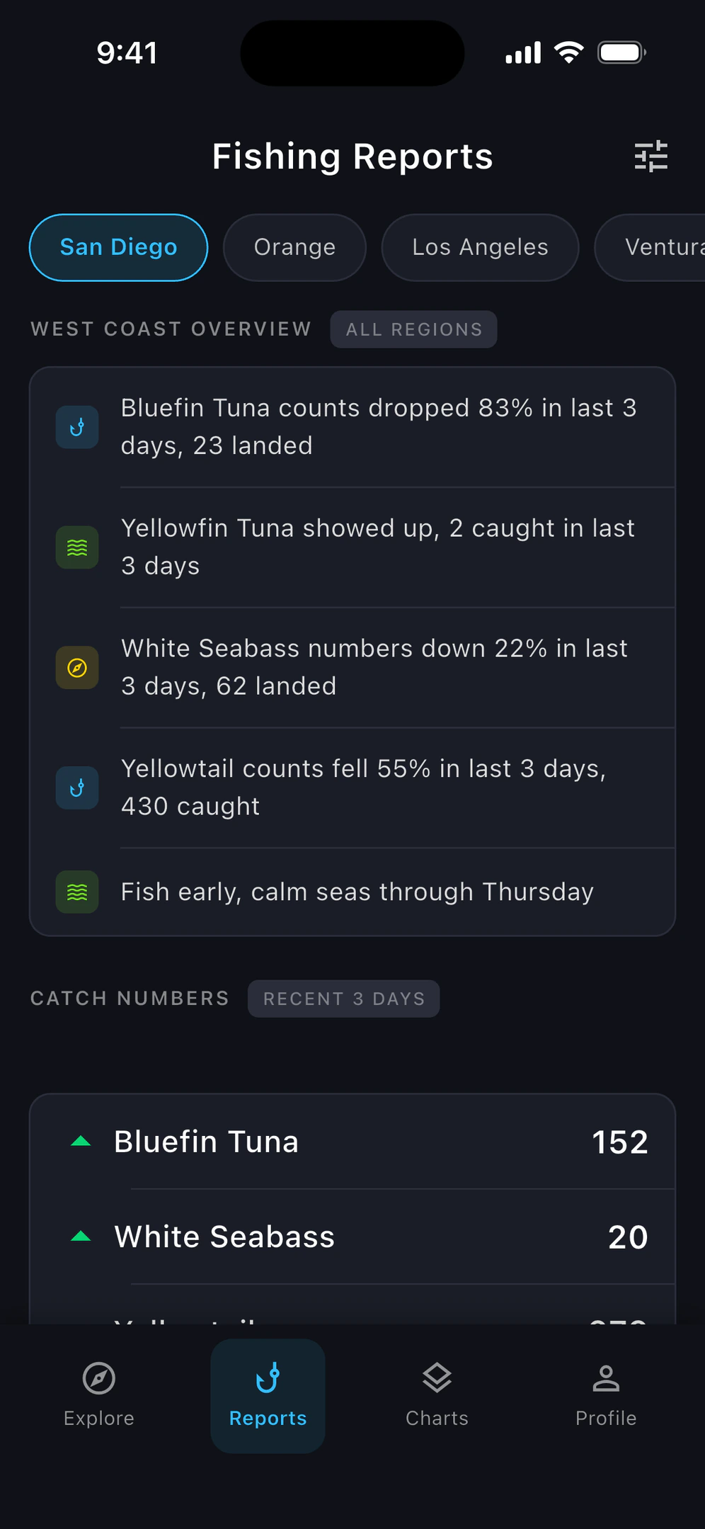
The last layer is human intel: what's actually being caught near your spot, read for
you and ranked prize-fish first. It arrives on two lanes. The clean lane is
SportFishingReport.com, scraped server-side every two hours across 11
West Coast regions (Washington down to Baja) and parsed with Jsoup into dock totals —
self-healing date drift, backing off politely on 429s.
The messy lane was the hard one. BD Outdoors is a forum behind
Cloudflare, so it can't be scraped from a server at all. A small Python scraper on my
own Mac reads the browser's
cf_clearance/session
cookies and POSTs to /v1/intel/ingest.
And forum chatter lies: the parser separates species that were mentioned from
species that were actually caught — catch phrases inside a window, excluding
chum, bait, freezer, and last-year references.
The result reads like a friend who scanned the docks for you: the prize fish lead, and
a mention never counts as a catch.
AI-written regional intel — prize fish first, landed separated from mentioned.
An earlier source, 976-tuna.com, was inflating and duplicating counts; I cut it and replaced
it with SportFishingReport. Everything dedupes on a SHA-256 fingerprint of
normalized
landing|boat|trip|date|anglers|sorted-species,
hardened after dedup collapsed distinct landings and punctuation quirks ("Halibut." vs
"Halibut") split identical ones. Species normalization and count/date parsing are
unit-tested; proximity uses a PostGIS GIST index on report geometries. Then Groq
(FishingIntelAiService,
llama-3.3-70b-versatile with an OpenAI fallback) extracts the caught species and a
mobile-sized TLDR per thread, flags real catch intel, and writes 3–5 punchy regional
insights that lead with the prize fish. It runs in background prefetch, off the request
path, and feeds the Highlights / Species Summary / Bait Status cards. Tuning the
48-hour-vs-5-day windows so it all reads as one list ordered by desirability was genuinely
fiddly.
Two lanes in, deduped and geo-indexed, then Groq turns chatter into a ranked, mobile-sized read.